Context

Say you are trying to reach an international number. It can cost a fortune to reach an operator on the other side of the world. You have limited funds and you wish to simulate a call centre system to estimate how likely you are to reach an operator before you run out of money.

Assumptions

It is critical to be extremely clear about the assumptions you are making when simulating a system. It should be clear in the analyst’s mind as to what the limitations are of the simulation. A simulation needn’t be overly complex, but it should be sophisticated enough to capture the core dynamics that are being investigated.

• Presume that it is a 24/7 line , but the number of call operators differs each shift.

• Assume that the call operators’ call resolution times are homogeneous within a given shift but each shift has a different mean waiting time. For example, on average you may need to wait longer when calling at night.

• Assume that people who are also waiting for an operator do not leave the queue. They wait until their calls are answered. This refers to the concept of reneging.

• We will also assume a ‘memoryless’ property to waiting in line. What this means is that if you have already been waiting \(T\) minutes (say 10 minutes in line), then this does not affect your chances of your call being picked up within the next t minutes. Simply put, the amount of time you have already been waiting does not influence your chances at all of your call being picked up.

Distributional Assumptions

A reasonable distribution to model the time a SINGLE call operator spends on an individual phone call is the Exponential distribution.

• Memoryless process: the Exponential distribution has this property discussed earlier.

• Independence between call operators.

• Exponential distribution is continuous and defined for positive variables.

Let there be two shifts per day: Day (8 am to 8 pm) and Night (8pm to 8am). I shall let the Day shift operators be more effective and thus they will have a lower mean call resolution time.

\(\lambda_{Operator}\) is the rate parameter which characterises the Exponential distribution. The average time a call operator will spend on a call in minutes is \(\frac{1}{\lambda_{Operator}}\).

Simulation Hyperparameters

Taking into account the previous two sections, we can set hyperparameters which will characterise the nature of the simulation

• Number of Day operators: 3
• Number of Night operators: 6
• Each call resolution time for a single Day shift call \(t_{Day} \sim E(\lambda_{day} = 1/3)\)
• Each call resolution time for a single Night shift call \(t_{night} \sim E(\lambda_{night} = 1/7)\)
• The cost per minute for calling an international number during the day is R31.85 and at night it is R27.94.

The respective distributions are plotted below:

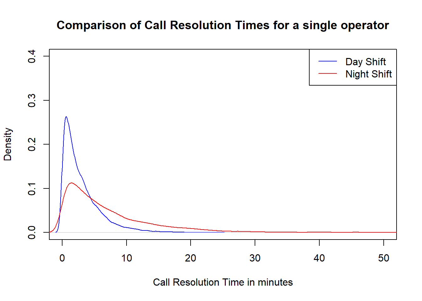
Variance in call resolution times at night is much higher than during the day. Since on average, the day time staff resolve calls more quickly, fewer staff are kept during this shift. Less experienced staff are kept on during the night shift.

Should you call at night when the international call fees are lower with more staff on duty or should you call during the day when the calls are more expensive but the fewer staff on duty are more efficient?

Simulating Waiting Times

Using the Exponential information for each call operator, a distribution for the amount of time that you would need to wait can be derived through simulation.

A function needs to be written to take into account:

• The number of call operators
• The call resolution rate of these operators

This function should return the minimum call resolution times for the N number of call operators. This represents the time you would have to wait if you were to stay on the line until someone was free to take your call. This shall be referred to as the “First Available” times.

call_pickup <- function(num_operators, pickup_rate){
  
  pickup_time <- rexp(n = num_operators,
                      rate = pickup_rate) %>% 
                      min()
  return(pickup_time)
}

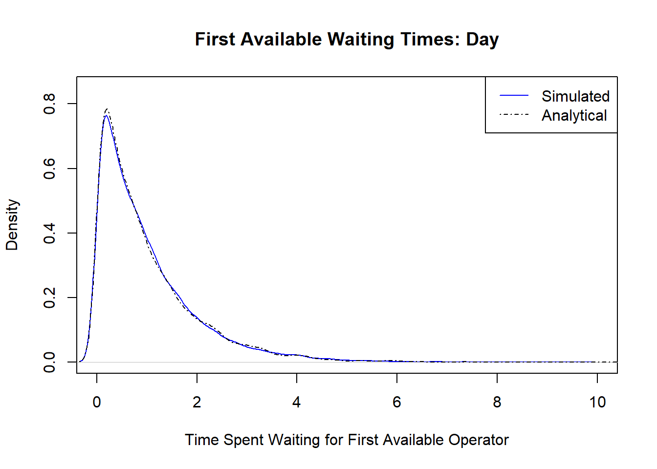
Let’s simulate the First Available waiting times for 10000 calls at each shift. What would be the distribution of waiting times?

Not surprising in that the minimum of Exponential variables is indeed an exponential distribution. We can see that the First Available waiting times are MUCH less variable now because you are waiting for the first available operator out of many. The difference between the First Available distributions is much smaller between shifts than the individual call resolution distributions.

Analytically Deriving Waiting Times

The First Available distributions is the same as simply calculating the distribution of the Minimum or rank 1 statistic for a sample of random variables.

In fact, this could be solved analytically using some basic probability theory surrounding cumulative density functions (CDFs). The thought process is to derive a distributional expression of the probability of observing a specific \(x^*\) as being the minimum value out of a sample of N data points.

\(\text{Cumulative Density Function(CDF)} = F(x^*) = Pr(X\leq x^*)\)

For it to be the minimum, we consider the probability of a value being greater than \(x^*\)

\(Pr(X\geq x^*) = 1 - F(x^*)\)

The above expression is the probability in which a random variable X has the same value or greater than \(x^*\). For \(x^*\) to be the minimum value from a sample draw of N random variables, each and every value needs to be greater than or equal to \(x^*\).

Probabilistically, assuming independence:

\(Pr(X_1, X_2 ... X_N \geq x^*) = (1 - F(x^*))^N\)

\(\text{In order to make the above expression into a CDF for the minimum:}\)

\(F(X_{min}) = Pr(X_{min}\leq x^*) = 1 - (1 - F(x^*))^N\)

We are nearly there. The last equation above shows the general expression for the CDF of the minimum order statistic out of a sample of \(N\) data points. Notice how no distributional assumptions were made in deriving this. In our case, the CDF for the Exponential distribution is substituted where \(F(x^*)\) stands. If we were dealing with Poisson variables for example, we would just need to substitute \(F(x^*)\) with the CDF of the Poisson distribution.

In order to achieve the density function, we would simply differentiate the expression with respect to the random variable \(x\).

The density distribution for the First Available Waiting times for the day shift is thus:

\(t^{(1)}_{day} \sim \lambda_{day}^{2} N\left(-e^{\lambda_{day}(-t^{(1)}_{day})}\right)\left(1-\lambda_{day} e^{\lambda_{day}(-t^{(1)}_{day})}\right)^{N-1}\)

We won’t need to use the density distributions as we can simulate variables from the CDF of the minimum order statistic using the Probability Inverse Transform method (PIT) method.

I shall skip over the explanation, but essentially variables from a desired distribution can be simulated directly through the use of uniform random variables

As a sanity check, the analytical and simulated First Available waiting times are the same.

first_order_sim <- function(n,rate){
  u <- runif(n =1)
  #Probability Inverse Transform of the CDF of the Min 
  -log(1-u)/(n*rate)
}

We can proceed to use the analytical result as it will be quicker to sample variables from this distribution rather than the simulation approach.

Will Anyone Answer Me?

We have an explicit analytical set of solutions for the First Available times. As a reminder, our central question is to answer:

Should you call at night when the international call fees are lower with more staff on duty or should you call during the day when the calls are more expensive but the fewer staff on duty are more efficient?

Under a fixed budget, let’s say R50, should we phone at night or during the day? I shall simulate the scenario 10000 times and calculate the success rates. To simplify matters, only two strategies are considered: phoning during the day or phoning at night.

One thing to keep in mind is that the total time spent on the phone is the sum of the First Available time and the call resolution time because you still need to discuss your issue with the operator.

call_scenario <-
  function(num, #number of  operators
           rate, #lambda characterising their performance
           budget = 50, #How much airtime you have to spend
           call_cost = 31.85, #cost per MINUTE
           period = 0 #0 is day and 1 is night
           ){

        #Simulate When An Operator Will Be Available
        waiting_time <- first_order_sim(n = num,rate = rate)
        #Simulate How Long it will take to resolve your issue
        resolution_time <- rexp(n = 1, rate = rate)
        #Calculate Money Spent Waiting for Call to be answered
        money_spent <- (waiting_time + resolution_time) * call_cost
        budget <- max(0, budget - money_spent)
        
        if(budget > 0){
          #IF you have money leftover and You didn't hang up, Call was Answered
          return(c(result = TRUE,period = period ))
        }else{
          return(c(result = FALSE, period  = period))
        }
        
}

The results are:

## The mean success rate for calling during the day is:  21.64 %

## The mean success rate for calling during the night is:  11.54 %

This is an interesting result in my opinion. We can see that when looking at the call resolution time of a single operator, the day shift staff are clearly superior. When considering the First available times, the time you would wait to reach the first available operator is more comparable between the two shifts however there is the possibility that you can wait up to 12 minutes when phoning at night. The night shift is heavier tailed than the day shift.

An important element to remember is that once you have reached the first available operator, they must still resolve your issue. Due to the huge discrepancy in success rates, it can be theorised that under the budget of R50, the additional time that you need to resolve your issue means that the superior efficiency per call operator during the day outweighs the cheaper phone rates during the night.

Although your chances are approximately doubled when phoning during the day, the overall success rate is quite low.

How much money would you need to budget for in order to guarantee that your issue will be resolved?

Money,Money,Money!

I consider a range of budgets starting from R0 up until R700. I calculate the mean success rate for budgets within this range. A useful package that I used for this is furrr. This allows you to easily run purrr functions like map() in parallel. I highly recommend checking this out as it is incredibly simple to use.

The results show that calling during the day approaches the asymptotic 100% success rate much faster than during the night. In order to achieve at least a 90% mean success rate, you would need to allocate on average R250 when calling during the day, but you would need to allocate R490 during the night in order to achieve the same mean success rate!

Unfortunately, it looks like my budget of R50 will be no good…

Main Ideas

This post has shown how one can create a simulation environment in order to ask specific questions. Sometimes one can figure out key elements analytically, but there is always simulation to help you find out the things you need to know.

The code is available on my GitHub so feel free to play around with the hyperparameters or use this as a basis for another scenario.

Thanks for reading!